DCSFQ inductor network
At a glance
| Property | Value |
|---|---|
| Project name | DCSFQ-inductor-network |
| Version | v1 |
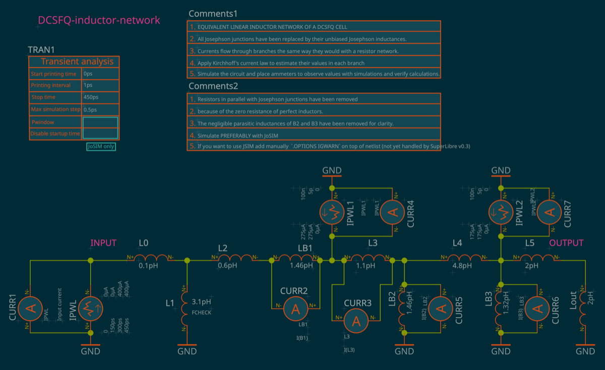
| Function | Linear inductor-network model of a DCSFQ cell — each Josephson junction at its steady-state operating point is replaced by its Josephson inductance, so the bias- and signal-current distribution can be computed and simulated |
| Josephson junctions | none — B1, B2, B3 are represented by the inductances LB1, LB2, LB3 |
| Inductors | 10 — series: L0, L2, LB1, L3, L4, L5; shunt to ground: L1, LB2, LB3, Lout |
| Josephson inductances | LB1 = LB2 = 1.46 pH (IC = 225 µA), LB3 = 1.32 pH (IC = 250 µA) |
| Input stimulus | 1 — IPWL, piecewise-linear current 0 → 400 µA |
| DC bias sources | 2 — IPWL1 = 275 µA, IPWL2 = 175 µA |
| Total device count | 13 (10 inductors + 3 current sources) |
| Current probes | 7 — input current, I(B1), I(L3), I(B2), I(B3), I(IPWL1), I(IPWL2) |
| Ports | none (self-contained network; the OUTPUT node across Lout is not probed) |
| Transient analysis | 0–450 ps, 1 ps print step, 0.5 ps max internal step (TRAN1) |
| Simulators supported | JoSIM (recommended); JSIM requires .OPTIONS IGWARN at the top of the netlist — the resistanceless inductor loops raise a topology warning that otherwise aborts the run |
Function
This example feeds a slowly rising current into an inductor network that models a DCSFQ cell whose Josephson junctions sit at their steady-state operating point. In that regime, each junction behaves as a linear inductor equal to its Josephson inductance LJ0 = Φ₀ / (2π·IC), and the cell reduces to a purely linear inductor network. Simulating it shows how the bias currents and the input signal current spread across the branches, and therefore which junction reaches its critical current first when a signal arrives. The full derivation is given in the SFQ generator example.
Expected results
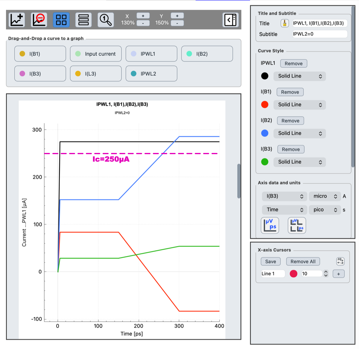
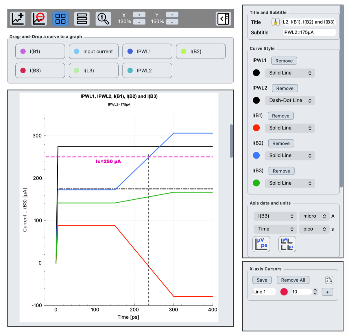
The graphs below show how the bias and signal currents distribute between the three Josephson inductances LB1, LB2 and LB3 (modelling junctions B1, B2 and B3), for two bias configurations. In both cases the input current is held at 0 until 150 ps, then ramps linearly to 400 µA between 150 ps and 300 ps.
Case 1 — IPWL2 = 0. Only IPWL1 = 275 µA biases the circuit. The dashed horizontal line marks the 250 µA critical current of B2 and B3. These currents can be compared with the values derived analytically in the SFQ generator example. I(B2) reaches the switching threshold at about t = 260 ps, while I(B3) stays far below it.
Case 2 — IPWL2 = 175 µA (black dash-dot line), the nominal operating value. The input ramp is the same. The graph shows both bias currents together with I(B1), I(B2) and I(B3). B2 now reaches its threshold slightly earlier, at t ≈ 240 ps, because of its higher initial bias current. B3 carries a much larger bias current, which would help it switch quickly once B2 has switched — a dynamic step that this quasi-static model cannot reproduce.
Bias and stimulus
| Source | Feeds | Current / waveform | Role |
|---|---|---|---|
| IPWL | INPUT node, through L0 | PWL: 0 µA until 150 ps, linear ramp to 400 µA between 150 ps and 300 ps, held to 450 ps | Emulates the rising input edge that triggers the DCSFQ cell |
| IPWL1 | node between LB1 and L3 | PWL 0 → 275 µA (rise over 0–5 ps, held to 100 ns) | Primary DC bias of the B1/B2 branch |
| IPWL2 | node between L4, L5 and LB3 | PWL 0 → 175 µA (rise over 0–5 ps, held to 100 ns) | Secondary DC bias; flows mostly through LB3 (B3) |
Josephson inductances
| Element | Models junction | Critical current IC | LJ0 = Φ₀ / (2π·IC) |
|---|---|---|---|
| LB1 | B1 | 225 µA | 1.46 pH |
| LB2 | B2 | 225 µA | 1.46 pH |
| LB3 | B3 | 250 µA | 1.32 pH |
Φ₀ = h/2e = 2.07 mV·ps = 2.07 pH·mA is the magnetic flux quantum. The junction shunt (damping) resistors and parasitic capacitances are omitted: they carry no current in the DC / steady-state limit, so they play no role in the current distribution.
Copyright (C) 2025-2026 SEFIRA. Licensed under the Apache 2.0 license.