First design with FrugalEDA¶

Basic example¶

First, launch LibrePCB which is inside the LibrePCB folder of the FrugalEDA folder chosen during installation. (On PC it is in the bin folder of LibrePCB folder). You should see something like that.

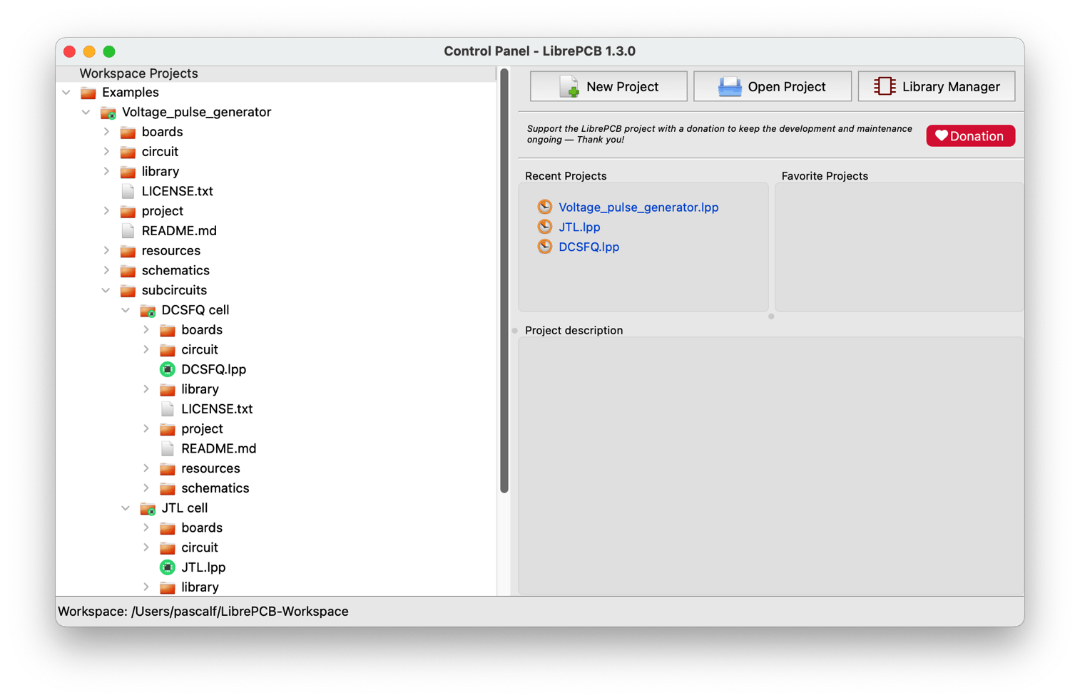
You will find in the Examples folder of the LibrePCB control panel a Voltage_pulse_generator project. This project contains two sub-circuits called DCSFQ cell and JTL cell. There are indeed two different cells used to make a voltage pulse generator: a DCSFQ cell and a JTL cell...

Superconductors library¶

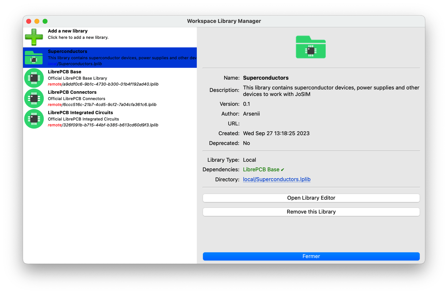
You can also click on the Library Manager icon of LibrePCB to make sure that the Superconductors library is recognized by LibrePCB. You should see it appearing:

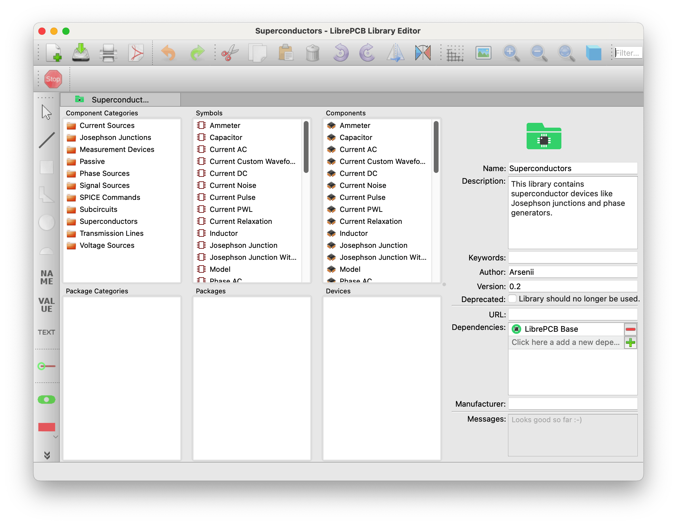
Double–click on it allows you to see its content. As you can see below, devices are categorized in a self-explanatory way. The SPICE Commands devices are some graphical blocks that contain syntax understood by simulators like JSIM or JoSIM, for instance to give the duration, step and stop time of a simulation. More to come about that on next releases.

Voltage pulse generator¶

Let's come back to the LibrePCB control panel. Double–click the Voltage_pulse_generator.lpp file to open the corresponding schematics. You should see something as shown below. It has been built with elements from the superconductor library. A good exercise is to build it yourself from scratch on a new project following this example. There are three monitoring probes Vout (for output voltage), Phase_out (for output phase) and Iinput ammeter that reads the current flowing through the IPULSE1 current pulse generator.

Note

An ammeter is usually placed in series with a device in a real electronic circuit. However in this case it is a virtual ammeter that simply checks the current flowing between the same two nodes as the ones of the IPULSE1 current source.

Voltage pulse generator schematics¶

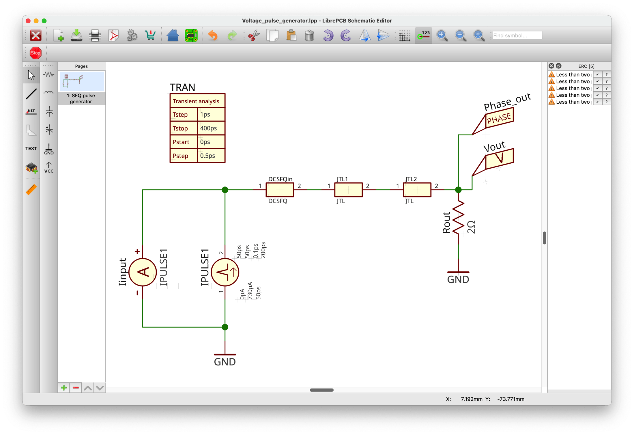
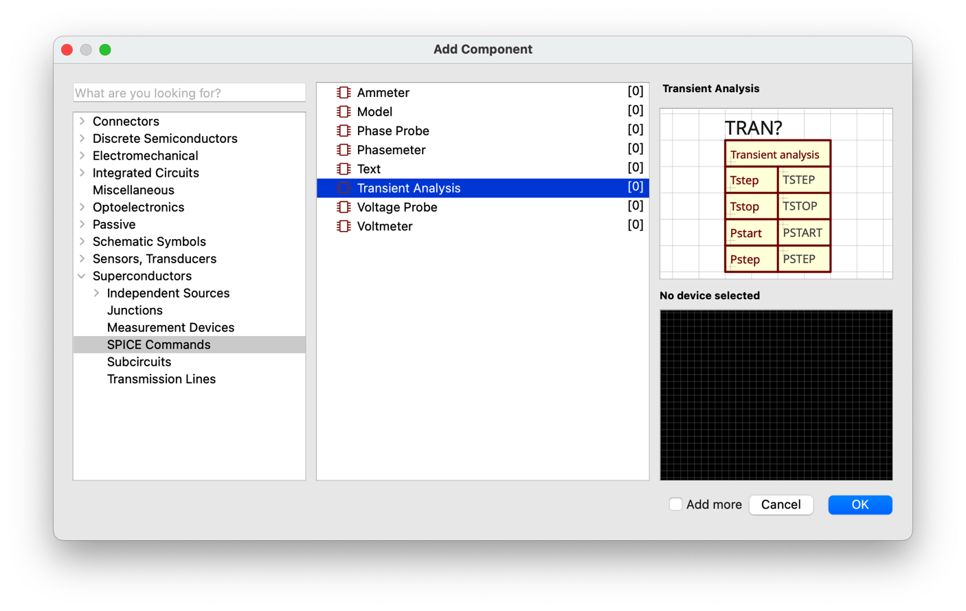
As mentioned just above, the TRAN table, which is a SPICE Commands element, gives the timing parameters needed for the transient time-domain simulation. It was placed on the schematics by clicking on the Add component icon on the left toolbar (or you can alternatively type the A key on your keyboard.) It is planned to make the simulation last 400ps starting from t=0ps, measure and plot the state of the circuit with a step of 1 ps. Internally the simulator solves equations with a time step not longer than 0.5ps to give sufficient smoothing and accuracy to the results.

Let us describe briefly the schematics of this simple circuit, which has been chosen because a voltage pulse generator is the first device needed to make superconducting digital electronics. Such circuit is used to generate picosecond-duration voltage pulses whose area is quantized due to quantum physics laws and equals the quantum of magnetic flux \(\phi_0=h/2e = 2.07 \ mV.ps = 2.07 \ pH.mA\).

Depending on the technology through the physical properties of the Josephson junctions the voltage pulse is typically of 1 mV amplitude and 2 ps duration. When this flux, or fluxon, is stored through a permanent current circulating in a superconducting loop the current is typically 1mA for a loop inductance of 2 pH. Due to their short duration it is possible to process pulses at high repetition rates corresponding to clock frequencies in the range of 100 GHz or more. Moreover there is no energy involved (the voltage is zero) when no pulse propagates in the circuit, similarly to the way the brain works (which explains the brain's low consumption of about 20 W).

These features make this technology very energy-efficient. The typical energy of a switching event is 10^-19J. It is also suitable to operate at very low temperatures close to the absolute zero because any energy waste corresponding to powers in the range of 10µW can totally spoil the operation of cryogenic cooling systems. Indeed they cannot hold too much power consumption due to their ultra-low energy efficiency of 10^-9 (typically 10µW of power is available at a physical temperature of 10 mK with 10kW necessary to run the cooling system).

The first task is to generate quantized voltage pulses, called SFQ pulses or Single-Flux-Quantum pulses. It is done by passing on the SFQ pulse generator a current at a low rate and of any waveform accessible by any commercial low-frequency signal generator. When the current crosses a certain threshold it induces the switching of a Josephson junction which is a very fast process in the picosecond range. The SFQ pulse generator acts like a Schmidt trigger better known in semiconductor electronics. It consequently generates a voltage pulse across the circuit. This voltage pulse can be used to do pulsed digital electronics at high speed. To generate a train of pulses the input current can be for instance a sinusoidal signal at the desired frequency (repetition rate) whose value passes the threshold once a period. But any proper periodic signal can do the work.

DCSFQ cell¶

The cell that does that is called a DCSFQ cell: it converts a low frequency signal (abusively called DC to evoke low frequencies) into an SFQ (Single-Flux-Quantum) signal, i.e. a very short voltage pulse in the ps range.

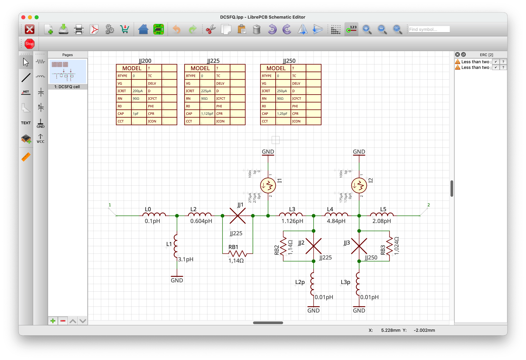
When one checks the voltage output of this cell one observes that the voltage pulse is not a neat and perfect pulse. It is rather shaky and comprises some oscillations, partly due to the non-perfect nature of the circuit components. By the way, it is a good exercise to insert voltage probes at different places inside the DCSFQ cell to display the DCSFQ voltage waveforms and confirm this assertion... It also allows to better understand its behaviour. You can see how the DCSFQ cell is built by double-clicking on the DCSFQ.lpp file from the LibrePCB control panel (this cell is placed inside the subcircuits folder). You will see the schematics shown below. The three tables were placed from the SPICE Commands elements of the Superconductors library. They give the physical parameters needed in the models to describe the behaviour of Josephson junctions.

JJ200 note

The JJ200 model is not used in fact, but it does not hurt simulations. It was used during the try and error iterations to optimize the cell parameters.

Tip

Circuit input and output are simply denominated by their node numbers (1 and 2 here) because this cell is used a a subcircuit. You can use names like IN and OUT. That will work well with JoSIM simulator, but not with JSIM which does not recognize the syntax.

JTL cell¶

A way to "clean" the DCSFQ output pulse is to pass it through a JTL cell, or Josephson Transmission Line cell, which acts as a pulse repeater. It "absorbs" the incoming imperfect pulse and, in the same way as the DCSFQ cell, triggers a new pulse once its threshold is crossed. Its schematics is shown below.

By passing the output signal of the DCSFQ cell through two JTL cells placed in series one can obtain a clean final output signal which is fed to a \(2\Omega\) resistance to monitor its shape through a voltage probe Vout as shown on the *voltage_pulse_generator schematic above. You can consider that the two JTL cells taken together act as a buffer between the DCSFQ cell signal generator and the circuit to be placed later at the output.

You can also see on the schematic that a phase probe Phase_out is also placed at the same point to monitor the phase of the output signal, the phase being here the phase of the quantum wavefunction that models the behaviour of signals in a superconducting circuit. More to come about that later in another manual. To keep a relative intuition of what's happening in the circuit just accept that, when a Josephson junction "switches", its phase is increased suddenly, but continuously, by \(2\pi\). The voltage pulse is simply the derivative of the phase (mutiplied by a constant). You can then consider that a voltage pulse is simply the manifestation in our world of phase changes in the quantum world. It is a generalization of what is used in classical electromagnetism with Faraday's law.

The low frequency chosen current generator IPULSE1 generates a periodic triangular signal with a period of 200ps. Its amplitude of 730µA is sufficient to trigger the switching of the JJ2 Josephson junction of the DCSFQ cell. The JJ1 "escape" junction is placed to avoid having signals reflecting to the input signal generator due to impedance mismatches inside the circuit of when the input current goes down to zero and generates an anti-fluxon under the form of a negative voltage pulse.

LibrePCB usage¶

To know more about how to design circuits with LibrePCB you can get started with its Quickstart Tutorial or watch the videos on Youtube.

Schematics to SPICE netlist conversion¶

The JoSIM and JSIM simulators used for simulation of superconducting circuits are based on the SPICE syntax which uses netlists to describe the schematics. Netlists are used by simulators to build equations needed to simulate the circuit behaviour in the time domain. The open-source L2SPICE converter is used to convert the internal LibrePCB netlists into SPICE netlists. You can open it by double-clicking on L2SPICE from the L2SPICE folder of FrugalEDA directory.

Configuring L2SPICE default paths¶

First configure manually the LibrePCB input folder from the L2SPICE settings (this will be improved to be automatic in further FrugalEDA releases). The LibrePCB default directory for the current example is ~/LibrePCB-Workspace/projects/Examples/Voltage_pulse_generator of LibrePCB-Workspace directory placed by default in your Home directory.
Then configure, also manually, the output folder for L2SPICE converted netlists. By default they should be placed inside the L2SPICE-Workspace folder which is by default in your Documents directory. For the curent example the chosen path is ~/Documents/L2Spice-Workspace/Examples/SFQ_pulse_generator. The L2SPICE folders may have to be created if they don't exist yet.
You also need to indicate the directory for subcircuits used by the main circuit. The subcircuits directory, which must be converted beforehand, are automatically loaded during the conversion of the main circuit. The subcircuits directory is ~/Documents/L2Spice-Workspace/Examples/SFQ_pulse_generator/subcircuits.

Converting subcircuits¶

There are two LibrePCB cells schematics to convert into netlist SPICE format.

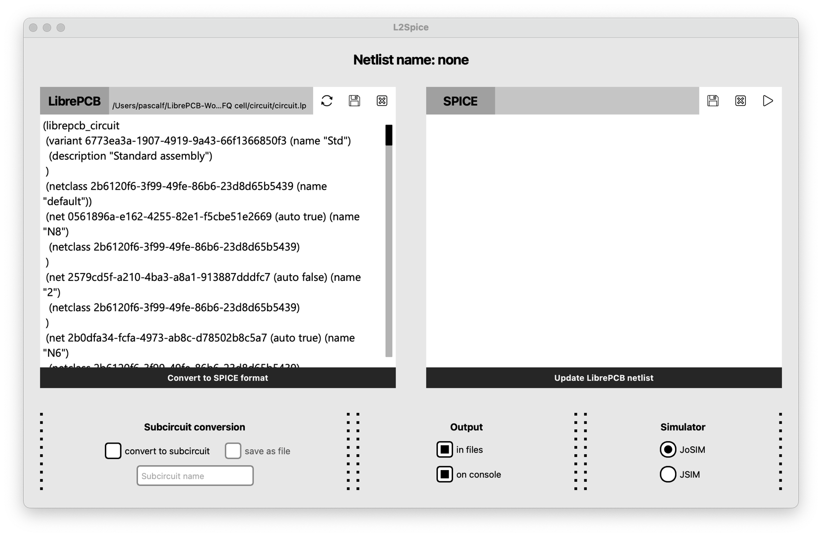
Start by opening the LibrePCB netlist of the DCSFQ cell. From the File menu of L2SPICE choose Open LibrePCB Netlist and find the circuit named circuit.lp in the following place~/LibrePCB-Workspace/Examples/Voltage_pulse_generator/subcircuits/DCSFQ cell/circuit/circuit.lp. You should see a LibrePCB netlist looking like this below.

To convert it, simply click on "Convert to SPICE format" at the bottom of the LibrePCB netlist and you will see the SPICE netlist appearing on the right part of the L2SPICE interface. This netlist could be directly simulated with JoSIM or JSIM if the DCSFQ cell input and output nodes were respectively connected to an input signal and an output load. There should be also some transient analysis parameters and some probes to tell the simulators what signal(s) to display. But the DCSFQ cell schematics, as designed, is to be used as a subcircuit only. Consequently these quantities must be present in the final circuit only. They are not needed for a subcircuit which can be considered simply like a 2-port device in this case. Then you cannot simulate this cell directly as designed.
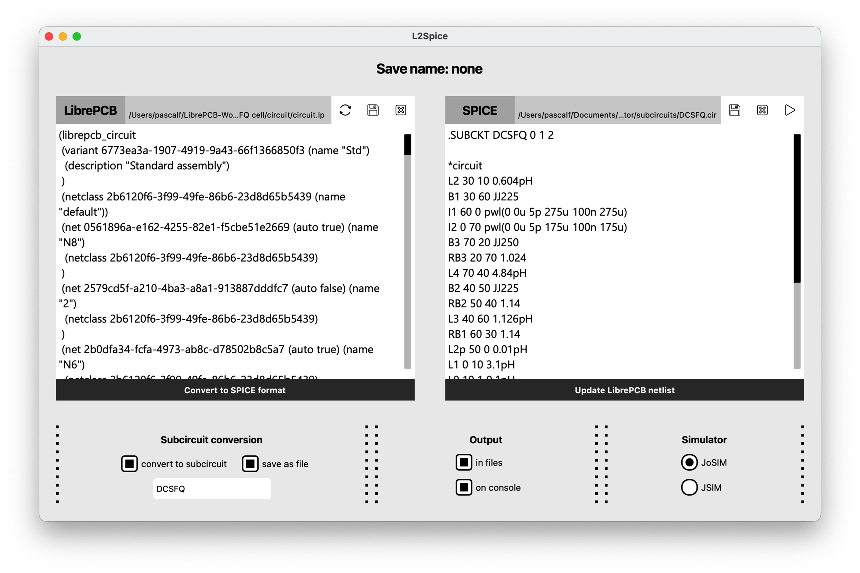
Let us then convert this LibrePCB netlist as a SPICE subcircuit. Check the "convert to subcircuit" and the "save as file" checkboxes and indicate the name of the subcircuit file, DCSFQ in this case, as it is the name indicated in the main schematics of the voltage_pulse_generator LibrePCB circuit. Then click again on "Convert to SPICE format" to convert the file and save it in a single action. You should see the converted netlist as shown below. You can notice the .SUBCKT and the .ENDS SPICE commands respectively placed at the beginning and end of the subcircuit SPICE netlist.

Warning after subcircuit conversion

Once the first subcircuit is converted and saved, clear the SPICE netlist window with the Close and clear icon at the top of the SPICE netlist window.

Then proceed the same for the JTL cell, saved under the JTL subcircuit name.

Converting the main circuit¶

The last conversion step is the conversion of the global circuit Voltage_pulse_generator. Proceed as before to open the LibrePCB netlist file at ~/LibrePCB-Workspace/Examples/Voltage_pulse_generator/circuit/circuit.lp.

Warning

Do not forget to uncheck the "convert to subcircuit" checkbox otherwise you will overwrite the last converted subcircuit.

Convert it by clicking on "Convert to SPICE format"
Save it explicitly with "Save SPICE Netlist As ..." from the L2SPICE File menu to the SFQ_pulse_generator folder in the L2SPICE-Workspace at ~/Documents/L2Spice-Workspace/Examples/SFQ_pulse_generator/SFQ_pulse_generator.cir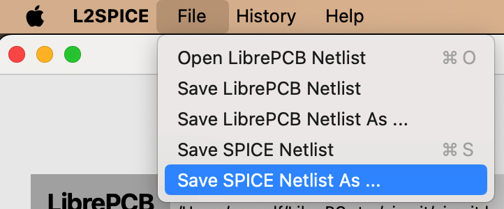

At the end of the process you should see this in the L2SPICE-Workspace folder. By default the file extension of SPICE netlists are .cir but JSIM supports .js as well (which creates confusion with javascript file extensions, so .js is to be avoided for new netlists).

The final circuit netlist is shown below. You can notice that L2SPICE has automatically included the netlists of the two subcircuits of DCSFQ and JTL cells at the top of the netlist. It also included at the end of the netlist the transient parameters of the TRAN block, which corresponds to the .tran SPICE command. It added a .PRINT command for each of the signal measurements probes incorporated on the schematics.

At last you can see that 3 lines (#6, 36 and 50) have been modified, and you should do the same manually from L2SPICE or any text editor. This is a known L2SPICE bug which is going to be fixed for next FrugalEDA release: sometimes the nodes of subcircuits or signal measurement probes are inverted in the SPICE netlist, which consequently does NOT correspond anymore to the LibrePCB netlist and drawn schematics.

.SUBCKT DCSFQ 0 1 2

*circuit
L2 30 10 0.604pH
RB1 30 60 1.14
*I1 60 0 pwl(0 0u 5p 275u 100n 275u) * L2SPICE CONVERSION MISTAKE
I1 0 60 pwl(0 0u 5p 275u 100n 275u)
L3p 0 20 0.01pH
RB3 20 70 1.024
L5 70 2 2.08pH
B3 70 20 JJ250
L4 70 40 4.84pH
B2 40 50 JJ225
RB2 50 40 1.14
L3 40 60 1.126pH
B1 60 30 JJ225
L2p 50 0 0.01pH
I2 0 70 pwl(0 0u 5p 175u 100n 175u)
L1 0 10 3.1pH
L0 10 1 0.1pH

.MODEL JJ225 jj(RTYPE=0 ICRIT=225u RN=90 CAP=1.125p)
.MODEL JJ200 jj(RTYPE=0 ICRIT=200u RN=90 CAP=1p)
.MODEL JJ250 jj(RTYPE=0 ICRIT=250u RN=90 CAP=1.25p)

.ENDS


.SUBCKT JTL 0 1 2

*circuit
RB2 10 50 1.024
B2 10 50 JJ250
L4 50 2 2.08pH
L3 50 40 2.06pH
*Ijtl 40 0 pwl(0 0u 5p 350u 100n 350u) * L2SPICE CONVERSION MISTAKE
Ijtl 0 40 pwl(0 0u 5p 350u 100n 350u)
L1p 0 30 0.01pH
RB1 30 20 1.024
L1 20 1 2.08pH
L2 20 40 2.06pH
B1 20 30 JJ250
L2p 0 10 0.01pH

.MODEL JJ250 jj(RTYPE=0 ICRIT=250u RN=90 CAP=1.25p)

.ENDS


*XDCSFQin DCSFQ 0 20 10 * L2SPICE CONVERSION MISTAKE
XDCSFQin DCSFQ 0 10 20
XJTL1 JTL 0 20 40
XJTL2 JTL 0 40 30
Rout 30 0 2
IPULSE1 0 10 pulse(0u 730u 50ps 50ps 50ps 0.1ps 200ps)

.PRINT NODEV 30 0
*.PRINT NODEP 30 0 * COMMENT THIS LINE OUT FOR JSIM simulations
.PRINT DEVI IPULSE1 

.tran 1ps 400ps 0ps 0.5ps
.end

Note

The .PRINT NODEP 30 0 must be commented out if you use JSIM because JSIM does not simulate circuit phases.

Simulating the main circuit¶

The next step is to simulate the main circuit, either with JSIM or JoSIM. You can download and install the simulators from the Open-source codes. There are also binaries available for JoSIM but you need to compile JSIM if you want to use it. Both simulators work with command lines only from a terminal. There is no available User Interface (UI).

Simulating with JoSIM¶

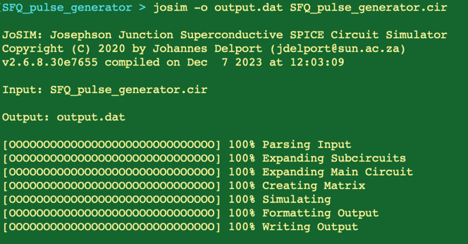
It is assumed that you correctly set your environment paths so that JoSIM is known. To check this just type josim-cli -h in the console, it should give you a short help manual and the JoSIM version

On Mac, from the console/terminal run the command josim-cli -o output.dat SFQ_pulse_generator.cirfrom the folder where the SPICE netlist is located.

On PC the default and preferred format for simulation results is .csv then proceed with josim-cli -o output.csv SFQ_pulse_generator.cir rather.

Simulation results should appear in the output.dat file on Mac, respectively output.csv on PC. The console (Terminal on Mac or PowerShell on PC) should display the content below.

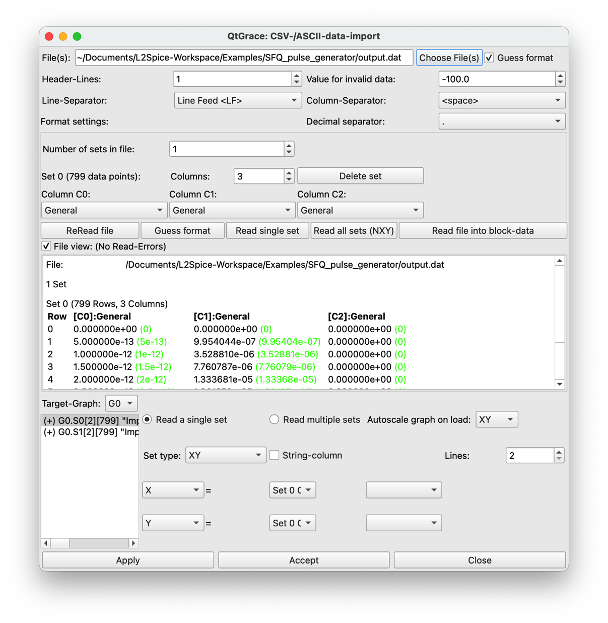
The beginning of the output.dat file is reproduced below for Mac. The phase is not shown (it was commented out in the neltlist).

time "V(30,0)" "I(IPULSE1)"
000000e+00 0.000000e+00 0.000000e+00
000000e-13 9.954044e-07 0.000000e+00
000000e-12 3.528810e-06 0.000000e+00
500000e-12 7.760787e-06 0.000000e+00
000000e-12 1.333681e-05 0.000000e+00
500000e-12 1.961973e-05 0.000000e+00
000000e-12 2.593246e-05 0.000000e+00
500000e-12 3.172758e-05 0.000000e+00
000000e-12 3.666687e-05 0.000000e+00

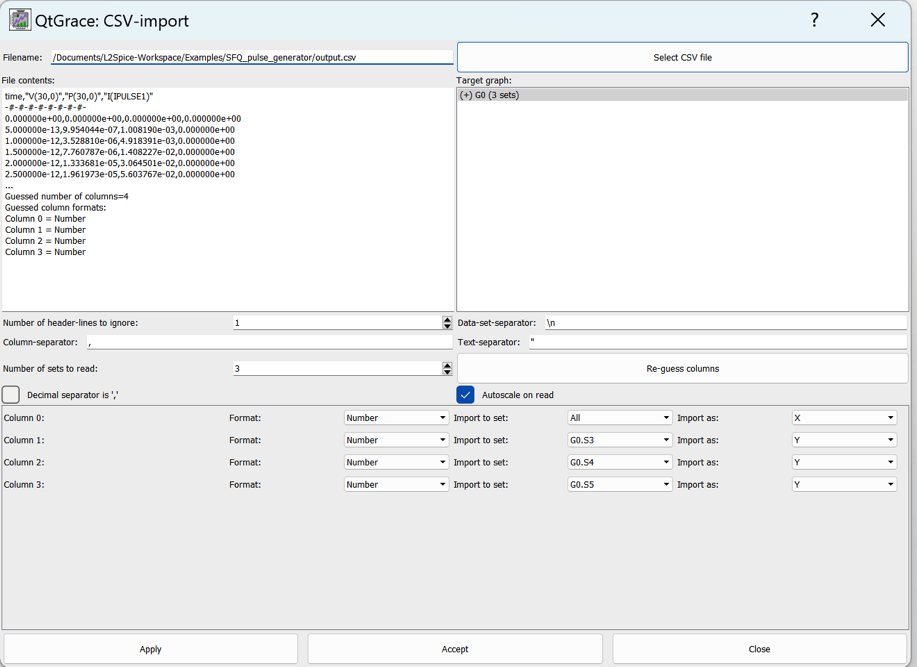
On PC the beginning of the output.csv file is reproduced below. The phase P(30,0) taken between nodes 30 and 0 is shown for the example on PC.

time,"V(30,0)","P(30,0)","I(IPULSE1)"
000000e+00,0.000000e+00,0.000000e+00,0.000000e+00
000000e-13,9.954044e-07,1.008190e-03,0.000000e+00
000000e-12,3.528810e-06,4.918391e-03,0.000000e+00
500000e-12,7.760787e-06,1.408227e-02,0.000000e+00
000000e-12,1.333681e-05,3.064501e-02,0.000000e+00
500000e-12,1.961973e-05,5.603767e-02,0.000000e+00
000000e-12,2.593246e-05,9.076746e-02,0.000000e+00
500000e-12,3.172758e-05,1.344792e-01,0.000000e+00
000000e-12,3.666687e-05,1.861876e-01,0.000000e+0

Simulating with JSIM¶

The procedure is similar. From the console/terminal run the command jsim -m output-JSIM.dat SFQ_pulse_generator.cir from the folder where the SPICE netlist is located.

Simulation results should appear in the output-JSIM.dat file. The console should display the content below.

SFQ_pulse_generator > jsim -m output-JSIM.dat SFQ_pulse_generator.cir
Filename for exported variables: output-JSIM.dat
.SUBCKT DCSFQ 0 1 2
*CIRCUIT
L2 30 10 0.604PH
RB1 30 60 1.14
*I1 60 0 PWL(0 0U 5P 275U 100N 275U) * L2SPICE CONVERSION MISTAKE
I1 0 60 PWL(0 0U 5P 275U 100N 275U)
L3P 0 20 0.01PH
RB3 20 70 1.024

............. [this central part skipped]

B1 20 30 JJ250
L2P 0 10 0.01PH

.MODEL JJ250 JJ(RTYPE=0 ICRIT=250U RN=90 CAP=1.25P)
.ENDS

*XDCSFQIN DCSFQ 0 20 10 * L2SPICE CONVERSION MISTAKE
XDCSFQIN DCSFQ 0 10 20
XJTL1 JTL 0 20 40
XJTL2 JTL 0 40 30
ROUT 30 0 2
IPULSE1 0 10 PULSE(0U 730U 50PS 50PS 50PS 0.1PS 200PS)

.PRINT NODEV 30 0
*.PRINT NODEP 30 0 * COMMENT THIS LINE OUT FOR JSIM SIMULATIONS
.PRINT DEVI IPULSE1 

.TRAN 1PS 400PS 0PS 0.5PS
.END

loop count      1206   predictor count   1207
timestep count    1206   LU count        11
Solve count     1330   solve ratio    41.330
LU size        41   LU percent filled  7.555
Non-zero elements   127   Fill-ins        12
Simulation ran 0.01 seconds.
This Stochastic extension to JSIM bought to you by
Julian Satchell, DRA(Malvern), UK. 
satchell@dra.hmg.gb
Our WWW page is at: www.dera.hmg.gb

The beginning of the output-JSIM.dat file is reproduced below.

time NV0 IPULSE1_I
000000000000000e+00 0.000000000000000e+00 0.000000000000000e+00 
000000000000000e-12 2.616423560424240e-06 0.000000000000000e+00 
000000000000000e-12 1.312821504519831e-05 0.000000000000000e+00 
000000000000000e-12 2.680258473516691e-05 0.000000000000000e+00 
000000000000000e-12 3.758153634071131e-05 0.000000000000000e+00 
000000000000000e-12 4.402918406645822e-05 0.000000000000000e+00 
999999999999999e-12 4.454192932163658e-05 0.000000000000000e+00 
999999999999999e-12 3.625967388718820e-05 0.000000000000000e+00 
000000000000000e-12 2.437909522465076e-05 0.000000000000000e+00 

Visualizing simulation results with QtGrace¶

It is possible to use any graphical tool to display the results. In case of large file, and when further analysis and data manipulation on large files is required, like Fourier transforms, Grace, and it's GUI version QtGrace, is a powerful tool. We will use it to display the results of the JosIM silmulations, the JSIM ones are similar.

Open QtGrace from the QtGrace folder of FrugalEDA directory (On PC it is placed in the bin directory).
Go to the menu Data-->Import-->CSV/ASCII ... (on Mac) or Data-->Import-->CSV ... (on PC)
Choose file output.dat on Mac or output.csv on PC, created by JoSIM.
You need to tell QtGrace that the first line of the file is a header line by choosing 1 in the Header-Lines field.
On PC make sure that the Column-separator field is a comma for csv format.
Then press the Reread file button on Mac (on Re-guess columns on PC) to verify that no error is displayed.
Press the Read all sets (NXY) button to import data on Mac. You should see 2 curves imported in the bottom left part as shown below. You can then close the import window.

On PC you should see a list of columns ready to be imported as shown below. Just click on the Apply button then close the import window.

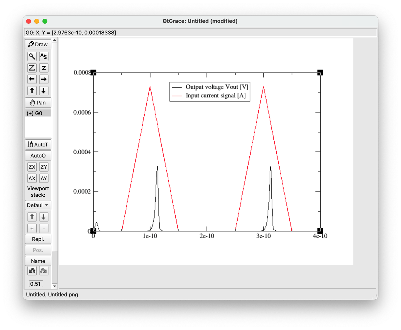
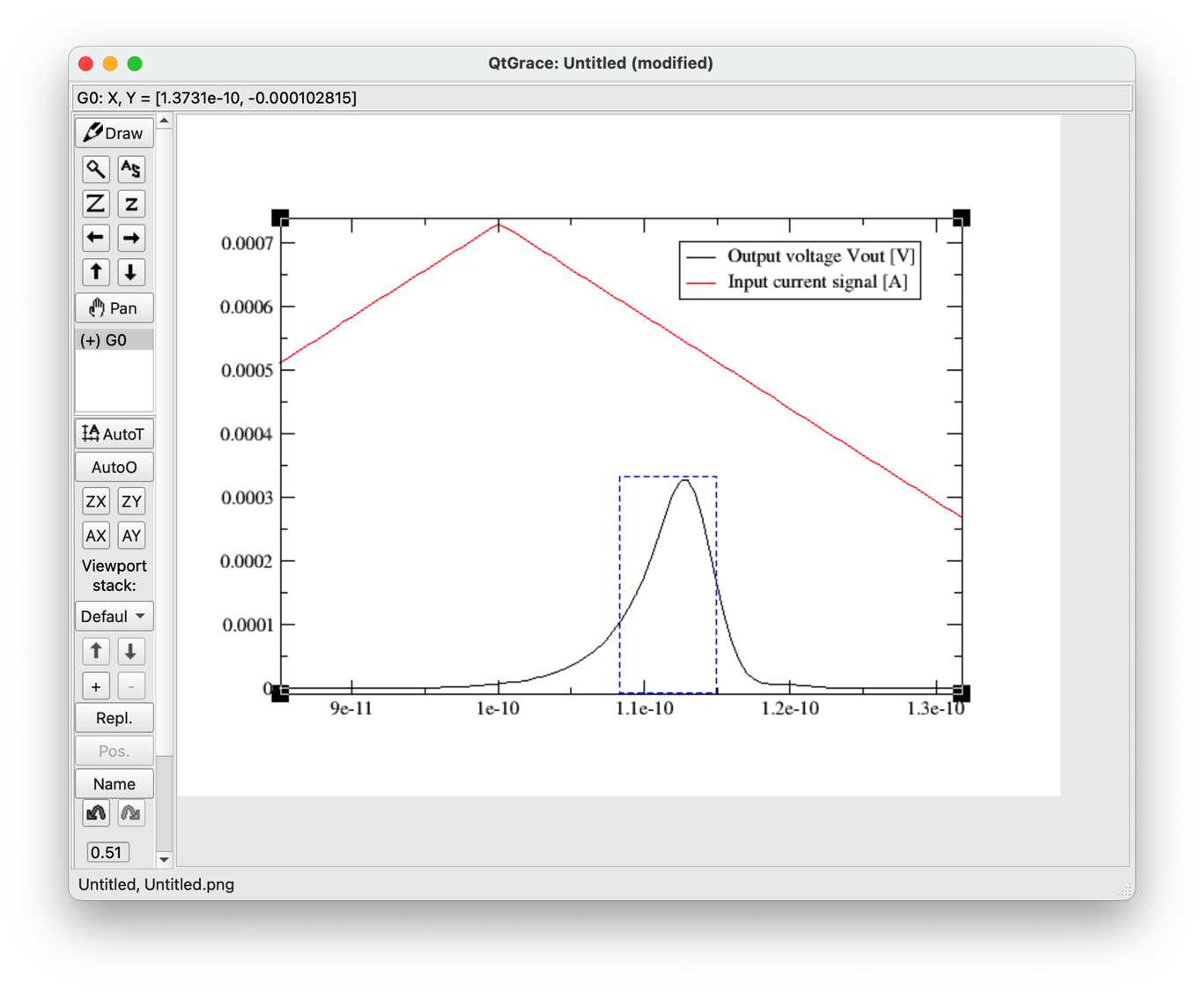
Finally you can see the signals as displayed below where a quantized voltage pulse is generated whenever the input current crosses the threshold of about 700 µA. The close-up view shows that the pulse area is roughly the same as the one of the 7 ps-wide dashed blue rectangle of 300µV amplitude. It corresponds to the quantized value of 2.07 mV.ps stated earlier.

On PC there is an additional curve showing the phase jumps each time a Josephson junction is switching, as shown below.
You can see the voltages by hiding the phase curve (menu View→ Set appearance... then right-click on the second graph in the Set appearance window then choose Hide ). Click finally on the Autoscale icon to display the input current and output voltage.

You are done with this first circuit example!